Derivatives, Critical Points, and Convexity of the Linear Regression Cost Function

Studying the Variation of Cost Function $J(w)$

We will focus on studying the variation of $J(w)$ with respect to $w$, by fixing the parameter $b$ to zero. That will allow us to later plot $J(w)$ in a simple 2D graph.

So for $b=0$, our model becomes $f_{w}(x) = wx$, and the cost function simplifies to:

$J(w) = \frac{1}{2m} \sum_{i=1}^{m} (wx^{(i)} - y^{(i)} )^2$

# In NumPy (b=0):
def compute_cost_jw(x, y, w):
    m = len(y)
    return (1 / (2 * m)) * np.sum((w * x - y) ** 2)

Computing the Derivative of the Cost Function $\frac{dJ}{dw}$

Let’s take the derivative of $J(w)$ with respect to w.

$$\frac{dJ}{dw} = \frac{1}{m} \sum_{i=1}^{m} x^{(i)}(wx^{(i)} - y^{(i)} )$$

Which is equivalent to:

$$\frac{dJ}{dw} = \frac{1}{m} \sum_{i=1}^{m} x^{(i)}(f_{w}(x^{(i)}) - y^{(i)} )$$

# In NumPy:
def compute_gradient_jw(x, y, w):
    m = len(y)
    return (1 / m) * np.sum(x * (w * x - y))

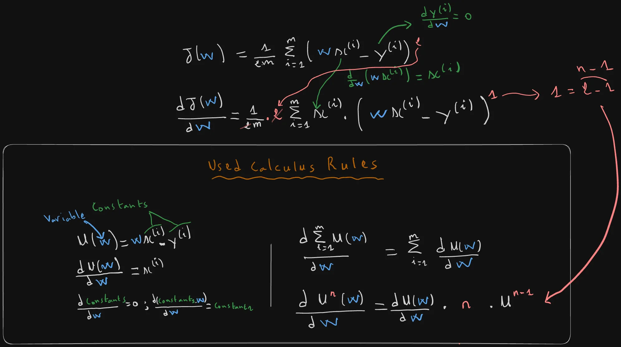
The derivation steps and the used calculus rules are described in detail in the following figure.

Step-by-Step Derivation Walkthrough (Optional)

Read this section if the previous figure wasn’t enough for you to understand the whole derivation process with every calculus rule explained in detail.

To find $\frac{dJ(w)}{dw}$, we pass the derivative operator inside the summation and apply the chain rule:

$\frac{dJ(w)}{dw} = \frac{1}{2m} \sum_{i=1}^{m} 2 \cdot \underbrace{\frac{d}{dw}(w x^{(i)} - y^{(i)})}_{\text{Inner Derivative}} \cdot (w x^{(i)} - y^{(i)})^{2-1}$

Evaluating the inner derivative yields $\frac{d}{dw}(w x^{(i)} - y^{(i)}) = x^{(i)}$. Canceling the constants gives:

$\frac{dJ(w)}{dw} = \frac{1}{\cancel{2}m} \cdot \cancel{2} \sum_{i=1}^{m} x^{(i)} \cdot (w x^{(i)} - y^{(i)})^1$

Which simplifies to our final form: $\frac{dJ(w)}{dw} = \frac{1}{m} \sum_{i=1}^{m} x^{(i)}(w x^{(i)} - y^{(i)})$

To compute the previous derivative, the following rules were applied:

Sum Rule:

Basically the rule states that the derivative of a sum of terms $u(w)$ is equivalent to the sum of derivatives $\frac{du}{dw}$:

$\frac{d}{dw} \sum_{i=1}^{m} u(w) = \sum_{i=1}^{m} \frac{du(w)}{dw}$

The Power Rule:

For a function $G(u)$ defined with a standalone variable $u$ as $G(u)=u^n$, the exponent $n$ drops down to the front, and the original power on top of $u$ gets reduced by $1$:

$G(u) = u^n \implies \frac{dG}{du} = n \cdot u^{n-1}$

The Chain Rule:

Let’s say that $G(u(w))$ is a composite (or nested) function defined as:

$G(u(w))= u^n(w)$ $w \to u(w) \to G(u(w))$

The derivative is calculated by multiplying the derivative of the outer function $dG$ with respect to the inner function $u$, by the derivative of the inner function $u$ with respect to its own variable $w$:

$\frac{d}{dw}[G(u(w))] = \frac{dG}{du} \cdot \frac{du}{dw}$

The Combined Form:

By applying both the chain rule then the power rule we get:

$\frac{d}{dw} [u(w)]^n = \underbrace{n \cdot [u(w)]^{n-1}}_{\text{ Power function } \frac{dG}{du} } \cdot \underbrace{\frac{du(w)}{dw}}_{\text{Inner Function} \frac{du}{dw} }$

Inner Derivative Evaluation:

In the expression $u(w) = w x^{(i)} - y^{(i)}$, we treat $w$ as the active variable as we are deriving with respect to it, while considering $x^{(i)}$ and $y^{(i)}$ as constants since they are totally independent from $w$.

So deriving $u$ with respect to $w$ gives us:

$\frac{du(w)}{dw} = \frac{d}{dw}(w x^{(i)}) - \frac{d}{dw}(y^{(i)}) = x^{(i)} - 0 = x^{(i)}$

$\frac{d}{dw}(y^{(i)}) = 0$ because the derivative of a constant is zero.

$\frac{d}{dw}(wx^{(i)}) = x^{(i)}$ Because the rate of change of a constant multiplied by the variable $w$ is the constant itself:

$\frac{d}{dw}(C1 w ) = C1$

Finding the Critical Point w*

To study the variation of the cost $J(w)$ and find its minimum, we look for the critical point where the derivative equals zero $\frac{dJ(w)}{dw} =0$

$$\frac{dJ(w)}{dw} = \frac{1}{m} \sum_{i=1}^{m} x^{(i)} \left( w x^{(i)} - y^{(i)} \right)$$

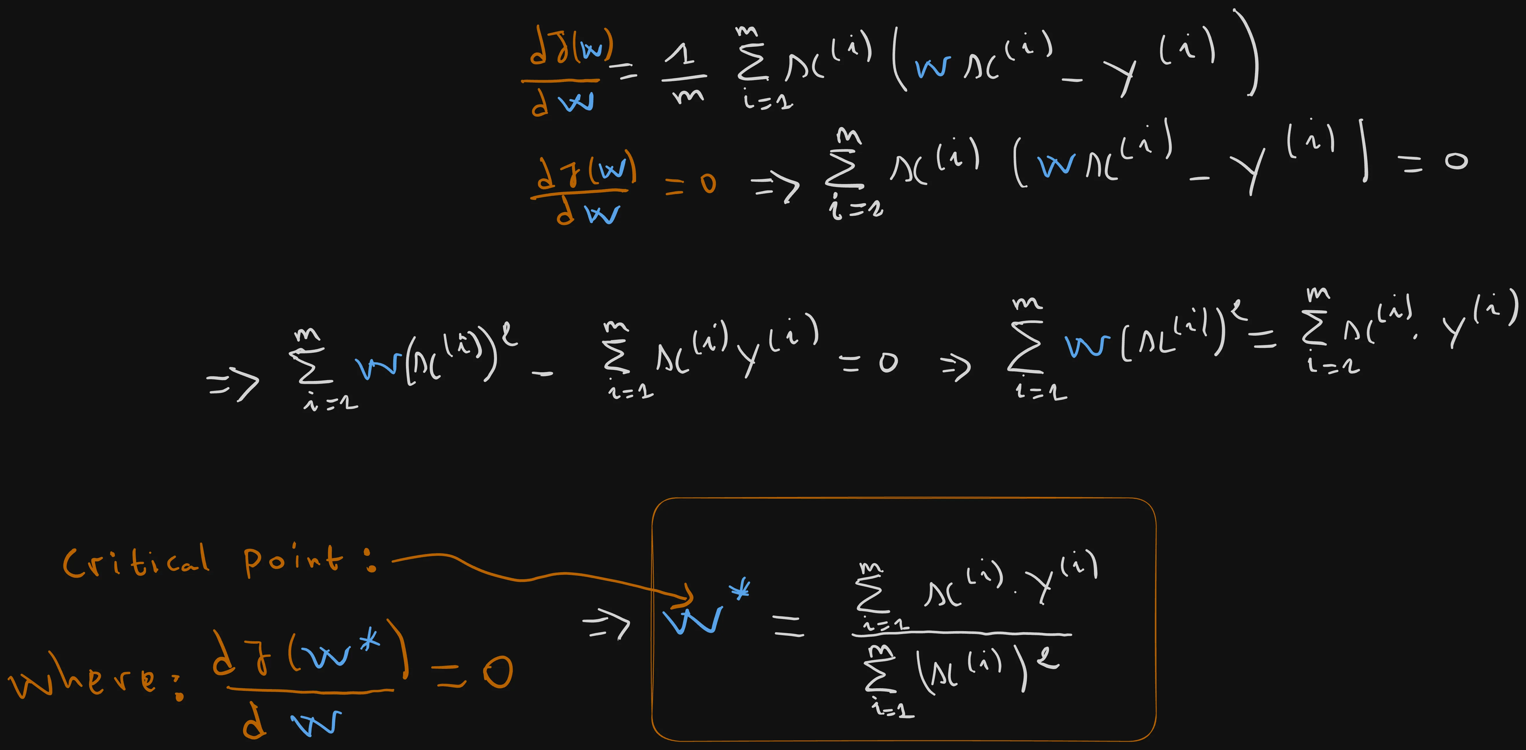
Setting the derivative to zero to find the critical point:

$$\frac{dJ(w)}{dw} = 0 \implies \sum_{i=1}^{m} x^{(i)} \left( w x^{(i)} - y^{(i)} \right) = 0$$

Expanding the terms inside the summation:

$$\implies \sum_{i=1}^{m} w \left( x^{(i)} \right)^2 - \sum_{i=1}^{m} x^{(i)} y^{(i)} = 0 \implies \sum_{i=1}^{m} w \left( x^{(i)} \right)^2 = \sum_{i=1}^{m} x^{(i)} y^{(i)}$$

Since $w$ is a constant factor relative to the summation index $i$, we can pull it out of the sum:

$$\frac{dJ(w)}{dw} = 0 \implies w \sum_{i=1}^{m} \left( x^{(i)} \right)^2 = \sum_{i=1}^{m} x^{(i)} y^{(i)}$$

After that we can divide by the ($\sum_{i=1}^{m} \left( x^{(i)} \right)^2$) term to isolate $w$.

$$\text{So the Critical point is: } w^* \text{ where } \frac{dJ(w^*)}{dw} = 0 \implies w^* = \frac{\sum_{i=1}^{m} x^{(i)} y^{(i)}}{\sum_{i=1}^{m} \left( x^{(i)} \right)^2}$$

# In NumPy:
def compute_w_star(x, y):
    return np.sum(x * y) / np.sum(x ** 2)

Variation Table of the Cost Function $J(w)$

$$\begin{array}{|c|ccc|} \hline w & w^* - 50 & w^* & w^* + 50 \\ \hline \frac{dJ(w)}{dw} & - & 0 & + \\ \hline & J(w^* - 50) & & J(w^* + 50) \\ J(w) & \searrow & & \nearrow \\ & & J(w^*) & \\ \hline \end{array}$$ $$\begin{aligned} w^* &= 5.913\dots \\ J(w^* - 50) &= 27758.43\dots \\ J(w^*) &= 11.58\dots \\ J(w^* + 50) &= 27758.43\dots \end{aligned}$$

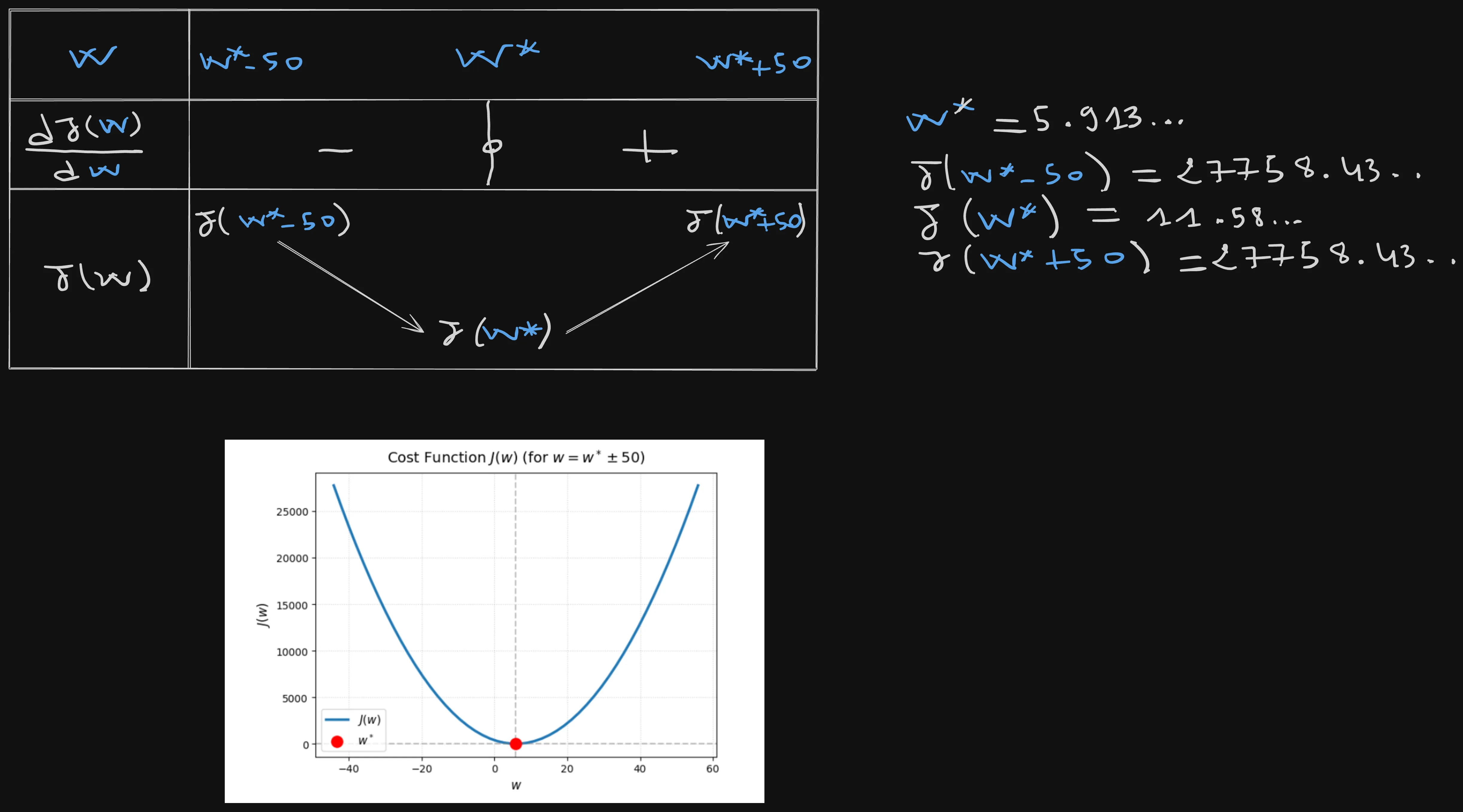
As presented in the figure and table above, when $w$ varies from $w^* - 50$ to $w^* + 50$, the derivative $\frac{dJ}{dw}$ is negative for values of $w$ between $w^* - 50$ and $w^*$.

It becomes zero at the critical point $w^*$, and then becomes positive after that.

The variation of $J(w)$ directly corresponds to the sign of its derivative: when the derivative is negative on a specific interval, $J(w)$ is decreasing, and when it is positive, $J(w)$ is increasing.

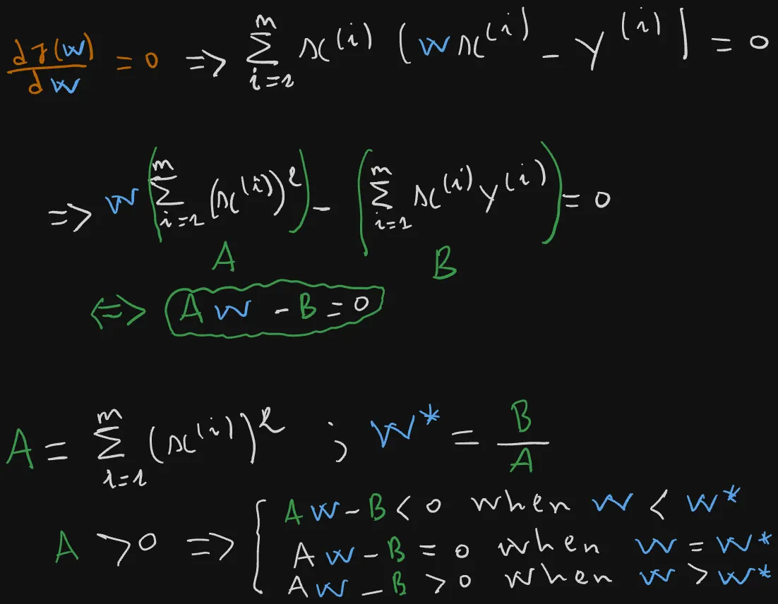
As we know from calculus, an equation of the form $Aw - B = 0$ is equal to zero when $w^* = B/A$. The sign of $Aw - B$ depends entirely on the sign of the coefficient $A$.

$\frac{dJ(w)}{dw} = 0 \implies w\sum_{i=1}^{m} \left( x^{(i)} \right)^2 - \sum_{i=1}^{m} x^{(i)} y^{(i)} = 0$

The previous equation is of the form $Aw - B = 0$, where:

$A = \sum_{i=1}^{m} (x^{(i)})^2 \quad ; B = \sum_{i=1}^{m} x^{(i)} y^{(i)} ; \quad w^* = \frac{B}{A}$

Because $A$ is a sum of squared terms, it is strictly positive ($A > 0$). When the leading coefficient $A$ is positive, the sign of the expression is determined directly by comparing $w$ to the critical root $w^*$:

$A > 0 \implies \begin{cases} Aw - B < 0 & \text{when } w < w^* \\ Aw - B = 0 & \text{when } w = w^* \\ Aw - B > 0 & \text{when } w > w^* \end{cases}$

The variation of $J(w)$ directly corresponds to the sign of its derivative: when the derivative is negative on a specific interval, $J(w)$ is decreasing, and when it is positive, $J(w)$ is increasing.

Proving Mathematically that $J(w)$ has a Convex Graph

As we’ve seen in the variation table, the graph of the cost function $J(w)$ forms a convex shape, or a ramen soup bowl shape if you like.

A convex graph in math is defined as follows: given two points belonging to the same graph $P_1$ and $P_2$, if we draw a line between them, it will always be either totally above the graph or totally below it.

In order to totally prove that $J(w)$ is a convex function, we need to calculate the second derivative $\frac{d^{2}J(w)}{d^{2}w}$:

$$\frac{dJ(w)}{dw} = \frac{1}{m} \sum_{i=1}^{m} x^{(i)} ( wx^{(i)} - y^{(i)} )$$ $$\frac{d^{2}J(w)}{d^{2}w} = \frac{1}{m} \sum_{i=1}^{m} (x^{(i)})^2 = A$$

The second derivative of $J(w)$ happens to equal $A$, the leading coefficient of the linear equation we derived when studying the first derivative.

Since $A$ is the sum of the squares of every input example $x^{(i)}$, which is totally independent of $w$, then $A = \frac{d^{2}J(w)}{d^{2}w}$ is always strictly positive.

This means that the first derivative $\frac{dJ(w)}{dw}$, which represents the slope of every point $(w,J(w))$, is always increasing.

It starts with an increasing negative slope when $w < w^*$, nullifies and intersects with the horizontal axis at $w = w^*$ (the critical point), and then keeps increasing with a positive slope for all values of $w > w^*$.

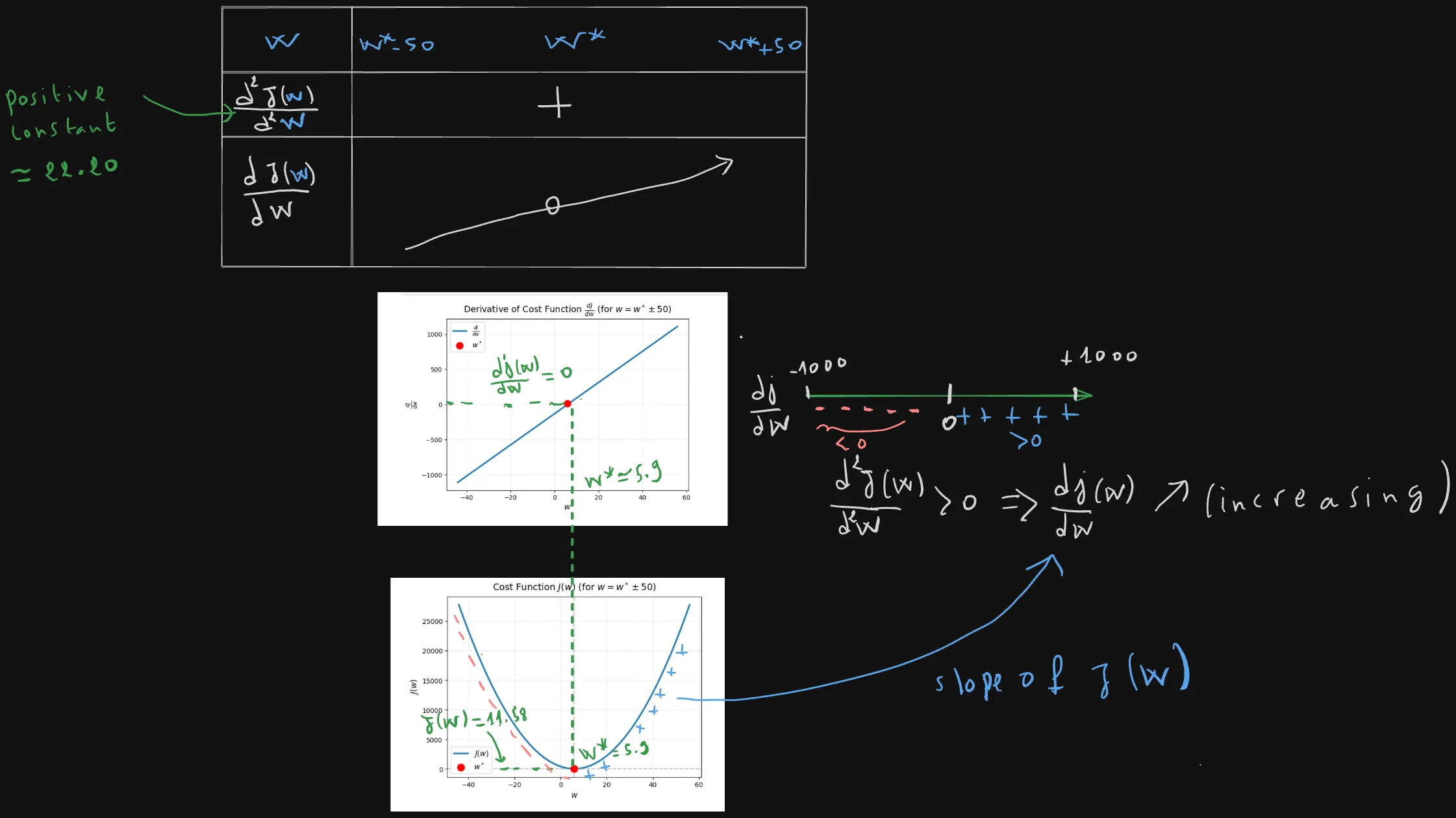
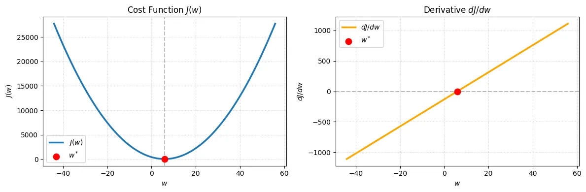
The fact that $\frac{d^{2}J(w)}{d^{2}w}$ is positive for all inputs $w$, and $\frac{dJ(w)}{dw}$ is equal to zero at point $(w^*,J(w^*))$ and changes its sign, mathematically proves that $J(w)$ is convex and that the point $(w^*,J(w^*))$ is its global, and only, minimum.

The left panel shows the $J(w)$ parabola on the Student Marks dataset, with the minimum marked at $w^*$. The right panel confirms the derivative $\frac{dJ}{dw}$ crosses zero exactly at that point.

Studying the Variations of the Cost Function $J(b)$

Now, let’s suppose that $w$ is equal to zero.

The model $f_{w,b}(x)$ becomes $f_{b}(x) = b$.

And the cost function simplifies to: $J(b) = \frac{1}{2m} \sum_{i=1}^{m} (b - y^{(i)} )^2$

# In NumPy (w=0):
def compute_cost_jb(x, y, b):
    m = len(y)
    return (1 / (2 * m)) * np.sum((b - y) ** 2)

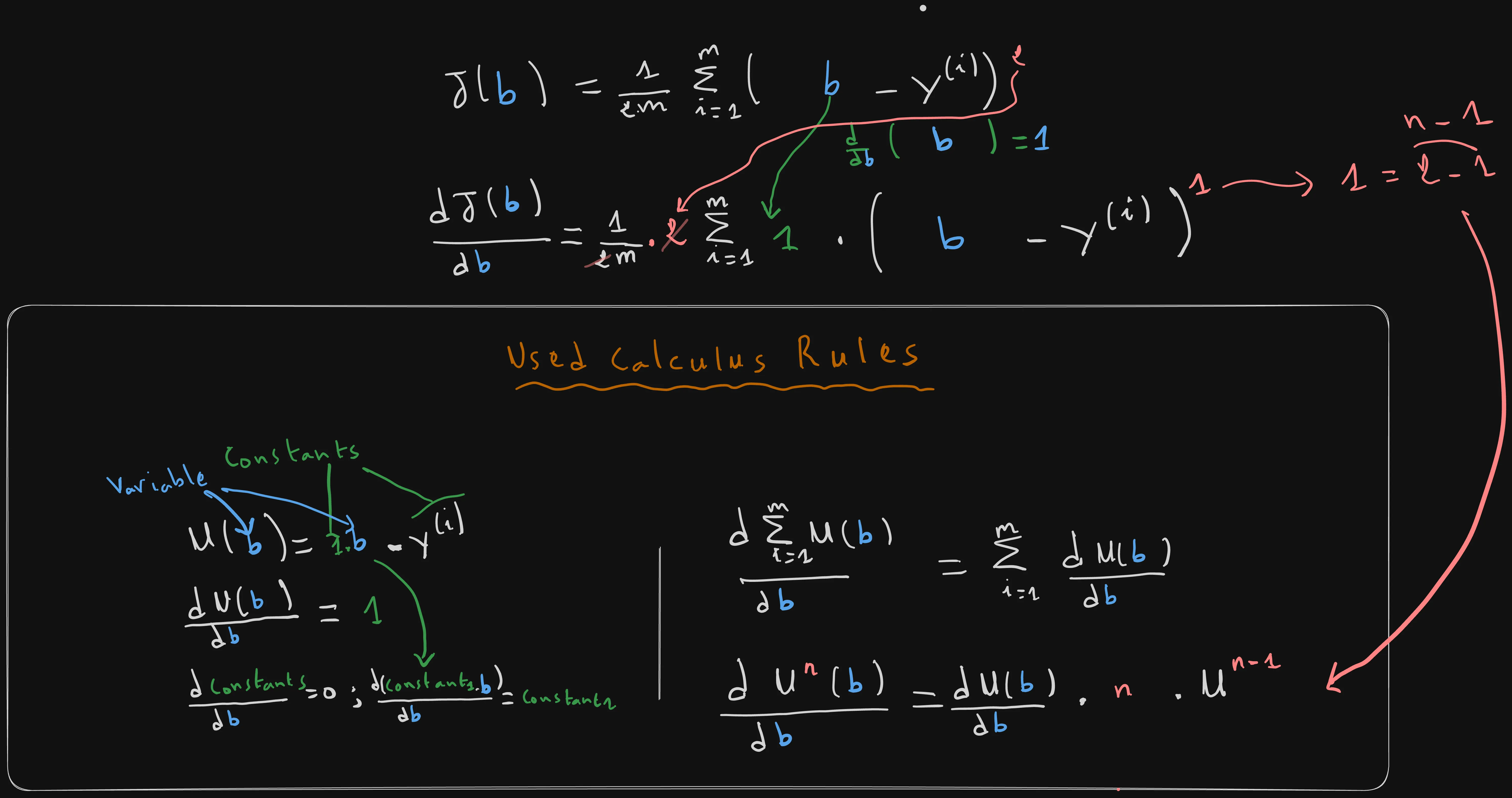
Let’s quickly calculate the derivative of $J(b)$, using the same calculus rules as before.

$\frac{dJ(b)}{db} = \frac{1}{m} \sum_{i=1}^{m} (b - y^{(i)} )$

# In NumPy:
def compute_gradient_jb(x, y, b):
    m = len(y)
    return (1 / m) * np.sum(b - y)

Finding the Critical Point b*

To study the variation of $J(b)$, we need to find its critical point, the point $(b,J(b))$ where the derivative $\frac{dJ}{db}=0$. Following the same derivation steps as before, we find that the critical point $b^*$ is actually the mean $\bar{y}$ of the target variable $y$:

$b^* = \bar{y} = \frac{1}{m} \sum_{i=1}^{m} y^{(i)}$

# In NumPy:
def compute_b_star(y):
    return np.mean(y)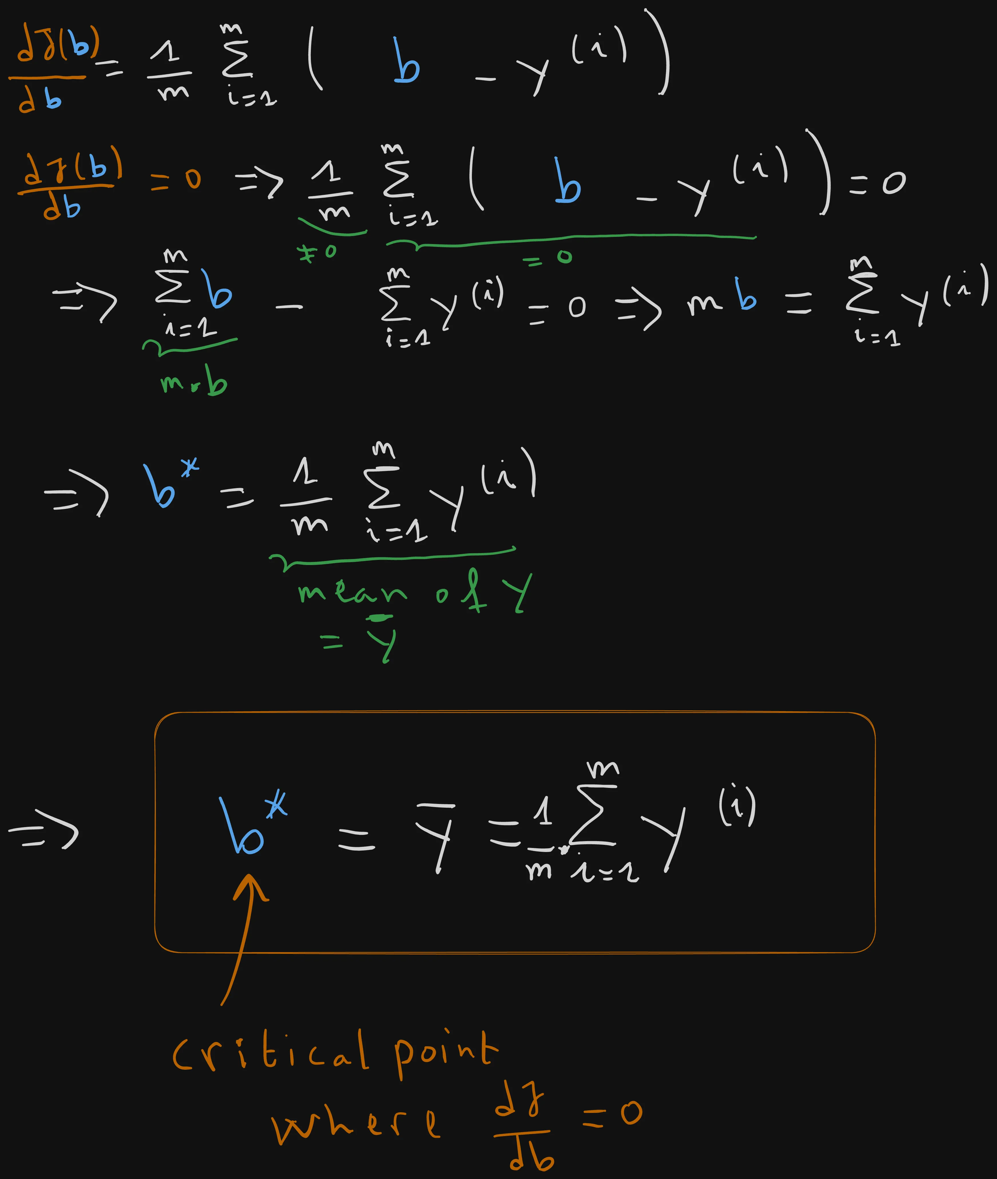

Variation Table of the Cost Function $J(b)$

$$\begin{array}{|c|ccc|} \hline b & b^* - 50 & b^* & b^* + 50 \\ \hline \frac{dJ(b)}{db} & - & 0 & + \\ \hline & J(b^* - 50) & & J(b^* + 50) \\ J(b) & \searrow & & \nearrow \\ & & J(b^*) & \\ \hline \end{array}$$ $$\begin{aligned} b^* &\approx 24.4 \\ J(b^* - 50) &\approx 1351.6 \\ J(b^*) &\approx 101.6 \\ J(b^* + 50) &\approx 1351.6 \end{aligned}$$

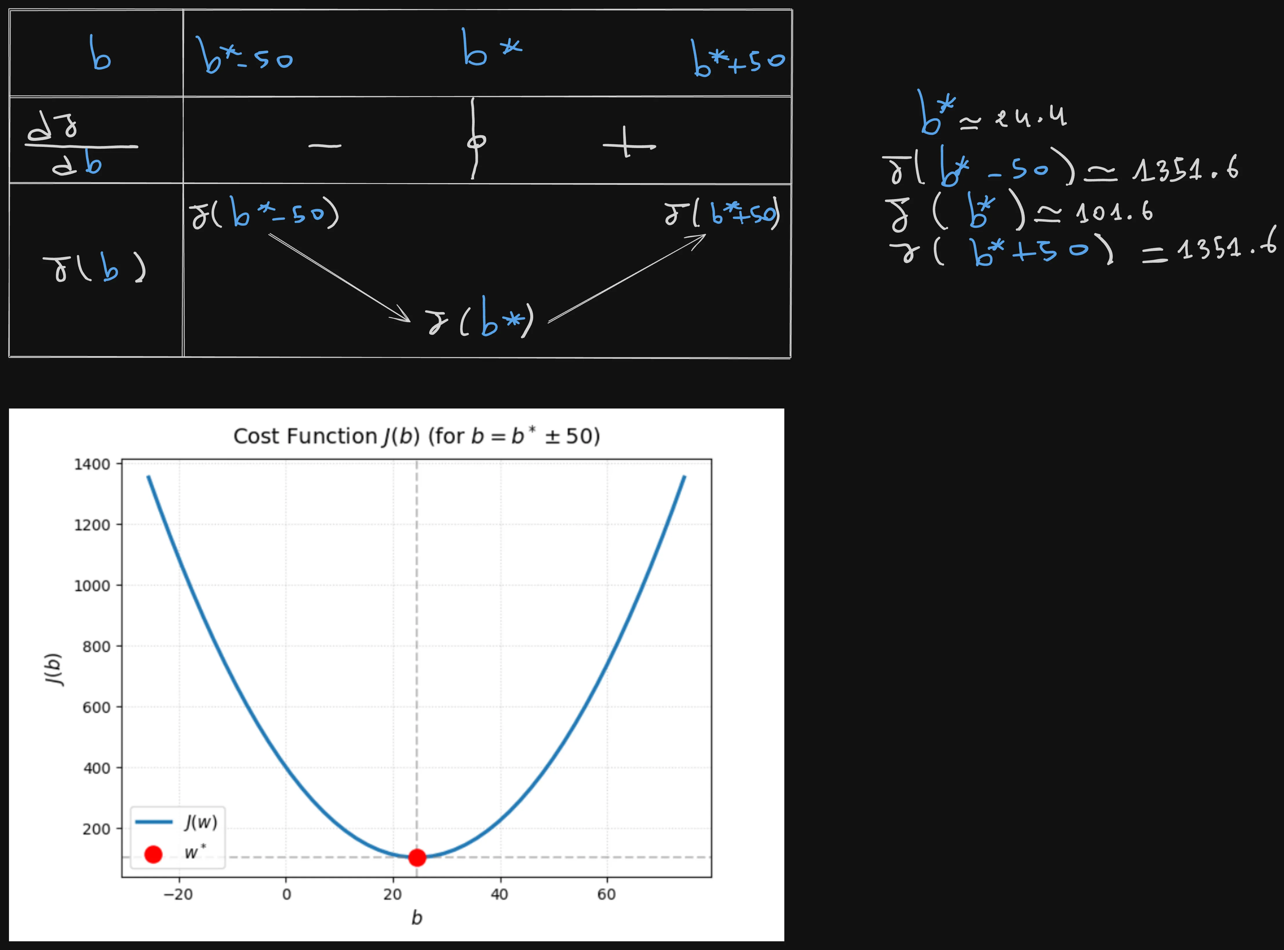
As presented in the figure and table above, when $b$ varies from $b^* - 50$ to $b^* + 50$, the derivative $\frac{dJ}{db}$ is negative for values of $b$ between $b^* - 50$ and $b^*$. It becomes zero at the critical point $b^*$, and then becomes positive after that.

The variation of $J(b)$ directly corresponds to the sign of its derivative. When the derivative is negative on a specific interval, $J(b)$ is decreasing, and when it is positive, $J(b)$ is increasing.

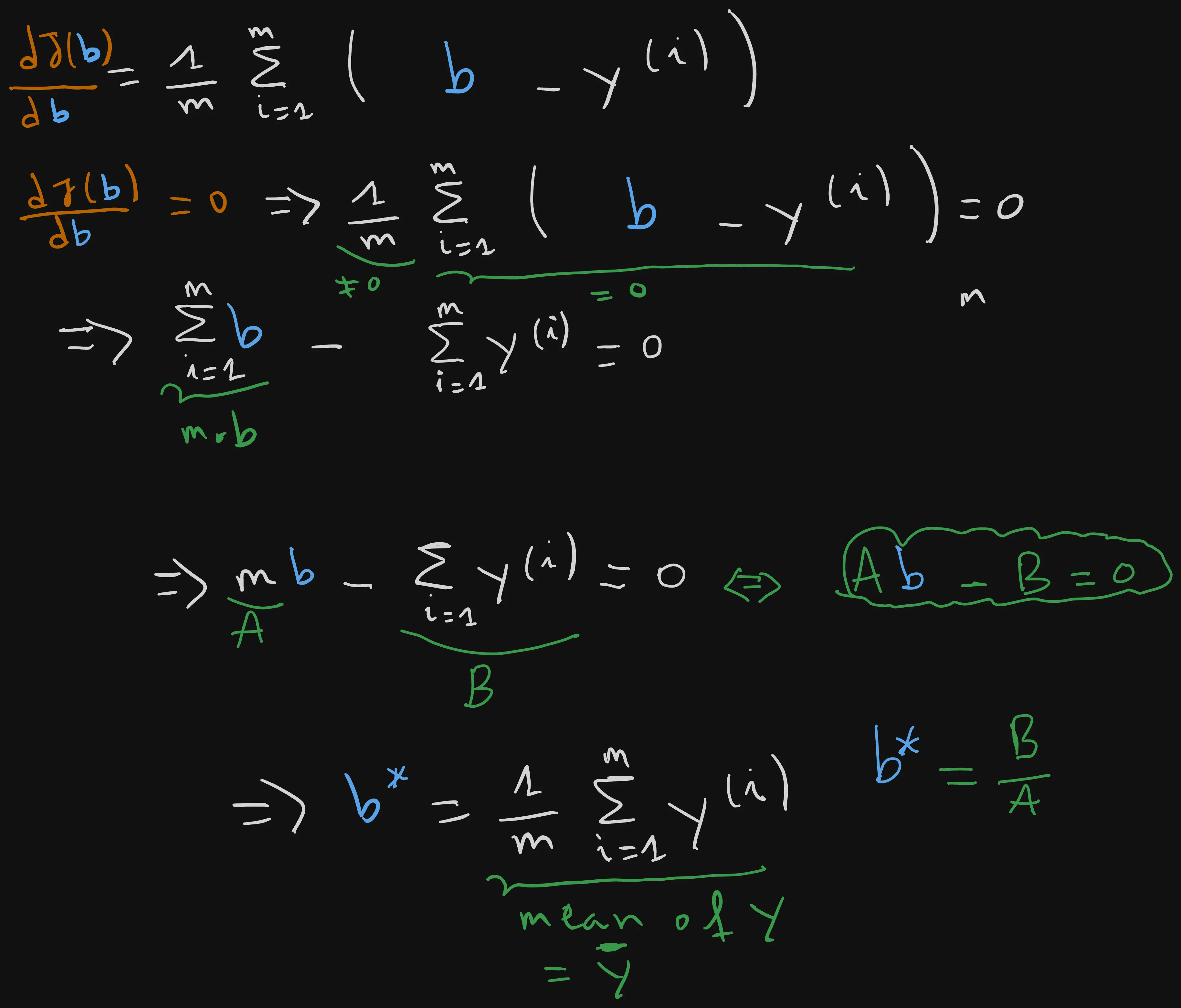
As we know from calculus, an equation of the form $Ab - B = 0$ is equal to zero when $b^* = B/A$. The sign of $Ab - B$ depends entirely on the sign of the coefficient $A$.

$\frac{dJ(b)}{db} = 0 \implies m \cdot b - \sum_{i=1}^{m} y^{(i)} = 0$

The previous equation is of the form $Ab - B = 0$, where:

$A = m \quad ; B = \sum_{i=1}^{m} y^{(i)} ; \quad b^* = \frac{B}{A}$

Because $A$ represents the number of training examples $m$, it is strictly positive ($A > 0$). When the leading coefficient $A$ is positive, the sign of the expression is determined directly by comparing $b$ to the critical root $b^*$:

$A > 0 \implies \begin{cases} Ab - B < 0 & \text{when } b < b^* \\ Ab - B = 0 & \text{when } b = b^* \\ Ab - B > 0 & \text{when } b > b^* \end{cases}$

Proving Mathematically that $J(b)$ has a Convex Graph

As we did with $J(w)$, let’s also prove that $J(b)$ is convex following the same steps.

The first step is to calculate the second derivative $\frac{d^{2}J(b)}{db^{2}}$:

$$\frac{dJ(b)}{db} = \frac{1}{m} \sum_{i=1}^{m} ( b - y^{(i)} )$$ $$\frac{d^{2}J(b)}{db^{2}} = \frac{1}{m} \sum_{i=1}^{m} (1) = \frac{1}{m} \cdot m = 1$$

Unlike the study of $J(w)$ where the second derivative matched the linear coefficient $A$, here the second derivative is a constant equal to 1.

Since 1 is strictly positive, the second derivative is always positive and entirely independent of both $b$ and the dataset values.

This means that the first derivative $\frac{dJ(b)}{db}$, which represents the slope of every point $(b,J(b))$, is always increasing.

It starts with an increasing negative slope when $b < b^*$, nullifies and intersects with the horizontal axis at $b = b^*$ (the critical point), and then keeps increasing with a positive slope for all values of $b > b^*$.

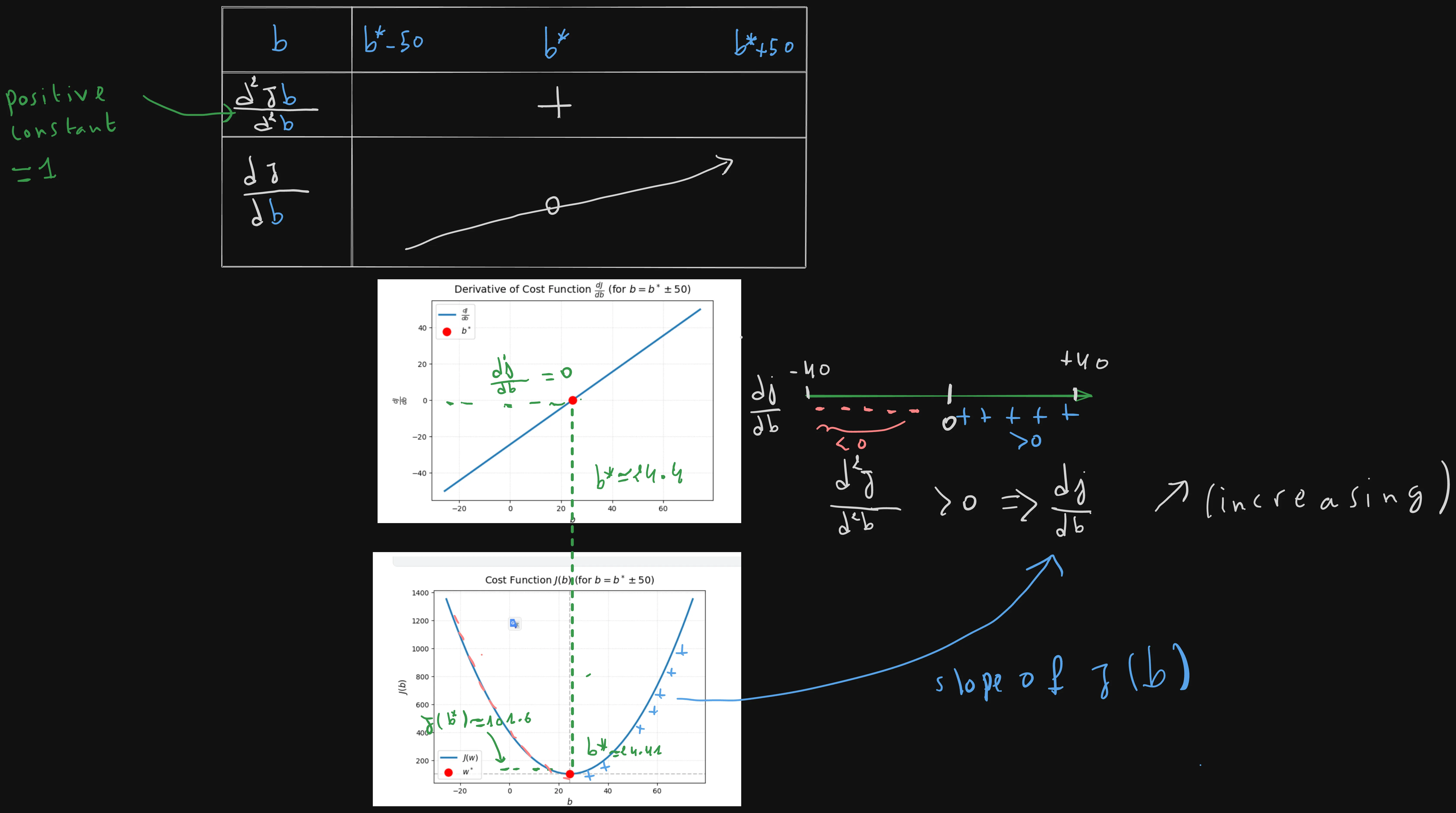
The fact that $\frac{d^{2}J(b)}{db^{2}}$ is positive for all inputs $b$, and $\frac{dJ(b)}{db}$ is equal to zero at point $(b^*,J(b^*))$ and changes its sign, also mathematically proves that $J(b)$ is convex, and that the point $(b^*,J(b^*))$ is its global, and only, minimum.

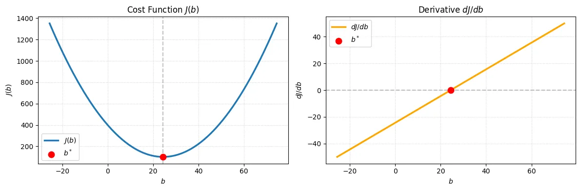
The left panel shows the $J(b)$ parabola on the Student Marks dataset, with the minimum at $b^* = \bar{y} \approx 24.4$. The right panel confirms the derivative crosses zero at that point.

Conclusion

In this article we’ve studied and proved that both $J(w)$ and $J(b)$ form a convex 2D bowl with a single and guaranteed global minimum $(w^*,J(w^*))$ and $(b^*,J(b^*))$ respectively.

In the first part we set $b=0$ to only study how $J$ varies with respect to $w$.

And in the second onewe set $w=0$ to only study how $J$ varies with respect to $b$.

But we never studied the full picture of it, when both $w$ and $b$ vary simultaneously.

In other words, we studied $J(w)$ and $J(b)$ but we’ve never actually studied the full cost function $J(w,b)$.

In the next article we will do that, and even scale the solution to any number of input features using the normal equation, and finally we will introduce the most important algorithm in machine learning “Gradient Descent”.Read Part 3: Gradient Descent Explained →

Just joining the series? Start from the beginning: Part 1: Linear Regression From Scratch