Cet article n'est pas encore disponible en français. Vous lisez la version anglaise.
Linear Regression From Scratch: The Model and Cost Function

Dernière mise à jour le
Introducing the Student Marks dataset
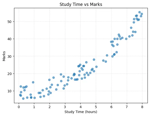
Student Marks Dataset: The data consists of two features including the study time and number of courses. In this blog article we will focus on how the students marks change with respect to the study time.
The Student Marks dataset consists of 3 attributes, two features “study time” and “number of courses”, and a target attribute “Marks”.
In this tutorial we will focus on studying how student marks increase, with respect to the number of hours they put into their studies.
The dataset contain training examples:
Scatter plot of the 100 training examples: study time on the x-axis, marks on the y-axis.
What is Linear regression
Linear regression means fitting a straight line to your data.
Training example notation
-
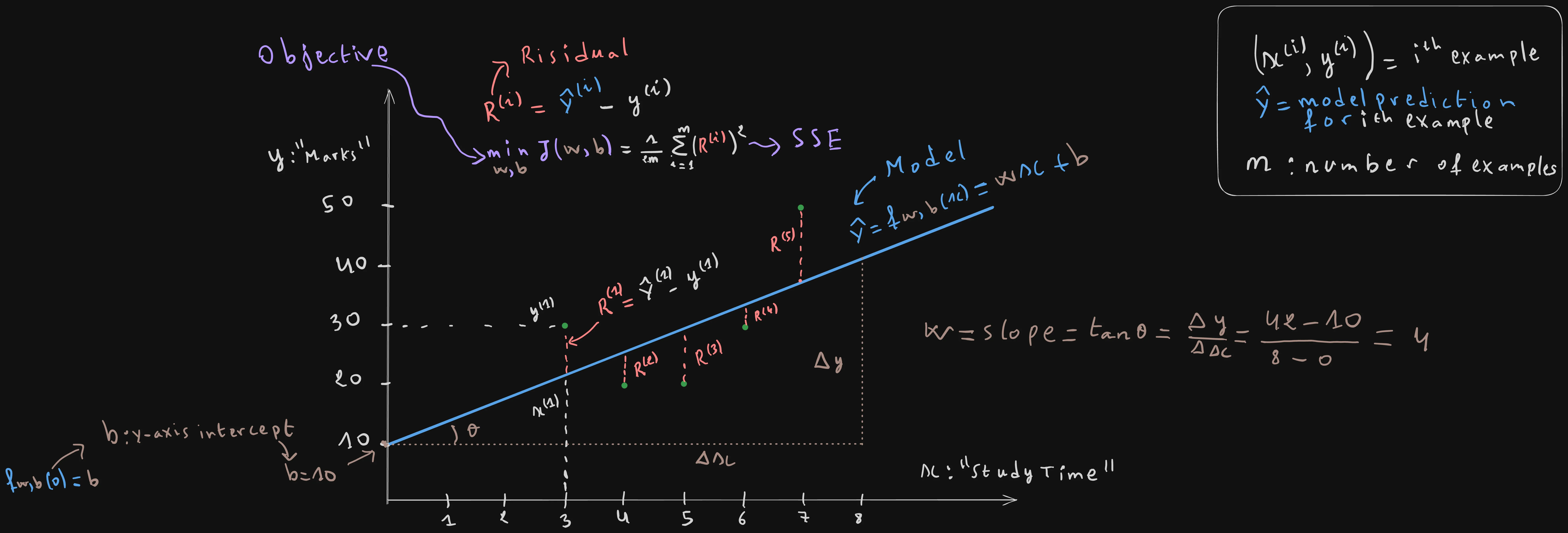
: A tuple representing the training example. Geometrically, it is the plotted point in the coordinate system, where represents the input feature (“study_time”) and represents the target output variable.
-
: Geometrically, this is the projection of the training point onto the X-axis.
-
: Geometrically, this is the projection of the training point onto the Y-axis.
-
: The total number of training examples.
E.g. the training example in the previous table () is represented by the tuple .
The linear regression model
Fitting a straight line to your data corresponds to finding a model:
Where:
- and correspond to any training example tuple .
- (pronounced “y-hat”) is the prediction of the model. This is also commonly referred to as the hypothesis, sometimes written as or .
- and are learnable parameters that control the slope of the line and its Y-intercept (intersection point with the Y-axis), respectively.
The model is called the linear regression model for one variable.
# In NumPy:
import numpy as np

def predict(x, w, b):
    return w * x + b
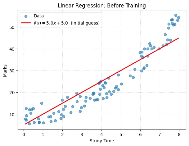
Before training, a rough initial guess already traces a line through the data, but it doesn’t fit well yet. Training will find the optimal and .
Understanding the slope parameter
controls the line’s slope. As shown in the figure below, the slope is the tangent of the directed angle from the x-axis to the line.
This is calculated for three cases: a high positive slope , a lower positive slope , and a negative slope .
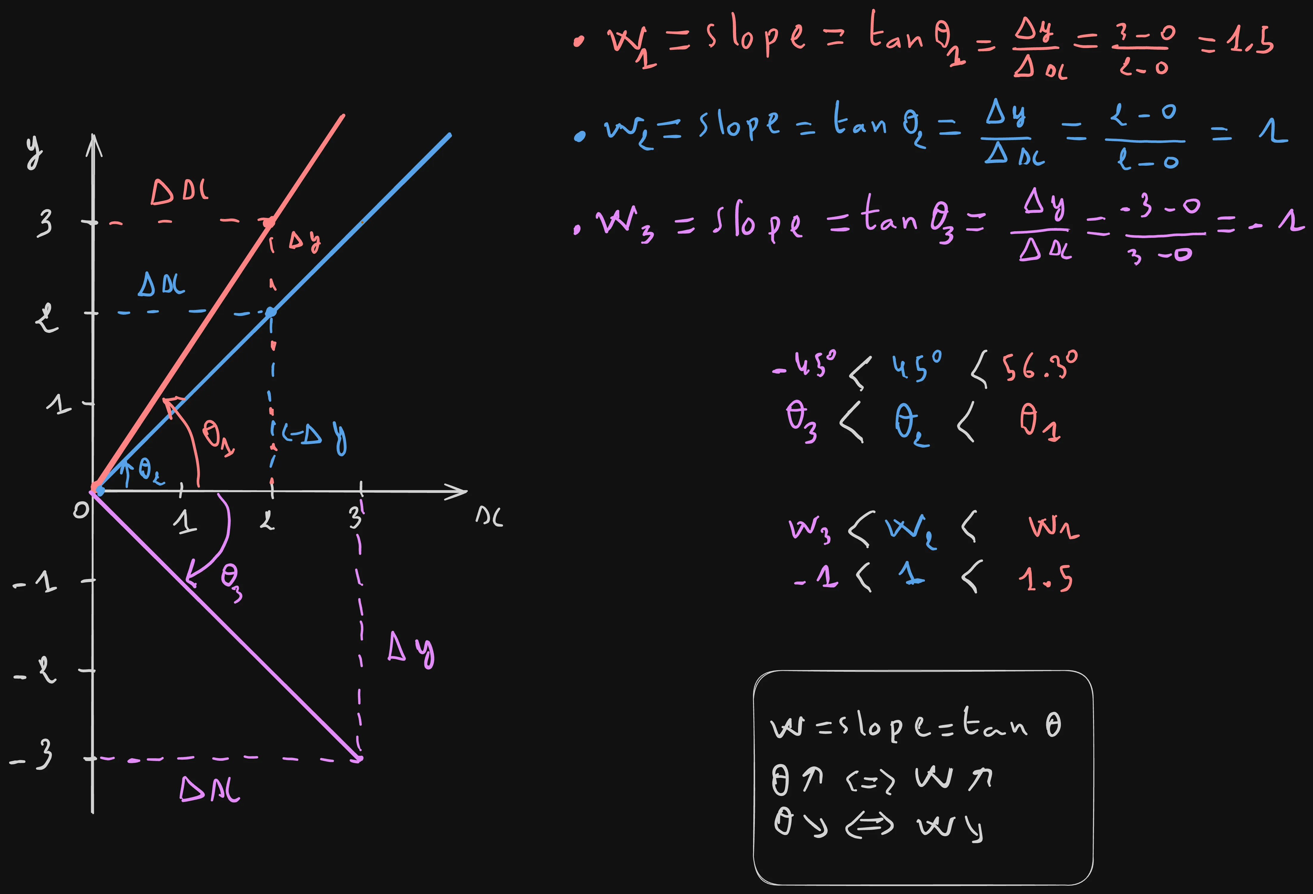
So in brief, the slope controls the direction of the line: when it’s positive, the line points towards the top-right.Whereas when it’s negative, it points down towards the right.
is calculated from two points on the line, and , by taking the ratio of the change on the Y-axis to the change on the X-axis .
Learning the model parameters
Linear regression is a model that learns how to fit a line to the data.
The learning itself needs a supervised learning algorithm that takes the training set consisting of examples , and learns the mapping from to . In our case this is a model that geometrically represents a line.
Learning the model actually corresponds to learning the coefficients or parameters and .
Evaluating parameters with an objective function
At each iteration the learning algorithm will try to find the optimal parameters and for the model.
To evaluate whether the parameters and are actually good or not in each learning iteration, we need to define an objective function.
Given the current parameters and , the cost function defines how well the current model is performing on the training set.
In math, this is an optimization problem, because we aim to find the optimal parameters and that either maximize or minimize the objective function.
When we try to minimize a function, the function is called a cost function. Whereas when we try to maximize it, the function is called: reward, utility, fitness, depending on the context where it’s used.
In linear regression we use a cost function which measures how inaccurate your linear model is at predicting target values .
Sum of squared errors
It’s known as SSE, or sum of squared errors. It measures how close the model’s prediction is from the ground truth target value for each training example in the training set of size .
That difference is measured by subtracting from and it’s referred to as the residual or the error.
is calculated by summing the squared residuals for each training example , and then dividing by the size of the training set multiplied by 2.
Dividing by or makes no big difference for the learning algorithm, but it simplifies the derivative of the cost function, which we will need in the next article of the series.
With and substituted in, the cost function expression for linear regression becomes:
# In NumPy:
def compute_cost(x, y, w, b):
    m = len(y)
    return (1 / (2 * m)) * np.sum((w * x + b - y) ** 2)
The figure below summarizes all what we talked about so far.
Conclusion
We now have a model parametrized by the slope and the Y-intercept that geometrically fits a line over the dataset and makes predictions about it.
And also a cost function that measures how wrong those predictions are.
A natural question that might come to your mind is: how do we actually find the values of and that minimize the cost function to its absolute global minimum?
Well, that’s exactly what we are going to learn in the next article, which is about: Read Part 2: Derivatives, Critical Points, and Convexity of the Linear Regression Cost Function
Cet article vous a plu ?
Je suis ouvert à de nouveaux postes, en télétravail ou à l'international. Si quelque chose vous a parlé ou si vous souhaitez collaborer, j'adorerais en discuter.
